Algodoo

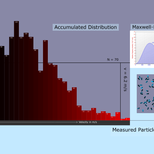
Exploring the 3D Maxwell-Boltzmann Distribution in a 2D World

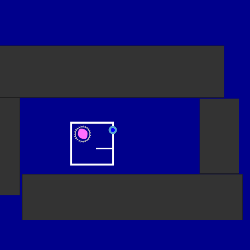
Welcome to this gas simulation! This setup demonstrates a diatomic gas in a two-dimensional space.

The Physics of Degrees of Freedom
The shape of a gas's speed distribution (known as the Maxwell-Boltzmann distribution) is entirely determined by its degrees of freedom, which are the independent ways a molecule can store energy.
- A simple monatomic gas in 1D has 1 degree of freedom (moving left/right).
- A monatomic gas in 2D has 2 degrees of freedom (moving along the X and Y axes).

Both can be observed in my previous simulation.

- This simulation: We are observing diatomic molecules in a 2D space. These molecules can move along the X and Y axes (2 translational degrees of freedom) AND they can spin around their center (1 rotational degree of freedom).

Mathematically and statistically, the universe doesn't care how the energy is stored. Because these molecules have exactly three degrees of freedom, their statistical behavior is identical to a standard monatomic gas flying around in our real, 3-dimensional world. The rotational energy simply acts as the missing third spatial dimension!

Reading the Graph
Because this system behaves mathematically like a 3D gas, the resulting graph looks a bit different from a 1D or 2D simulation. Look for these key qualitative features:
1. The curve starts completely flat at a speed of zero.
2. It features exactly two inflection points (where the curve changes from bending upwards to bending downwards, and vice versa).
3. A distinct peak representing the most probable speed.
4. The characteristic, long exponential decay tail towards higher speeds.


Note on Statistics: The universe is chaotic! To see the mathematical perfection of the curve with its peak, inflection points, and smooth exponential tail, you need to let the simulation run until it has collected approximately 10000 measured particles. The more, the better. With higher temperature you will need even more measurements to get a somewhat smooth graph. You can set a higher Temperature at the start of the sim by giving the molecules a little push. Or slow them down with activated air resistance. As with the previous sim you can scale the chart with scene.my.scaling (currently set to 3).